冲毕业第六七八周记录

https://zhuanlan.zhihu.com/p/25998937

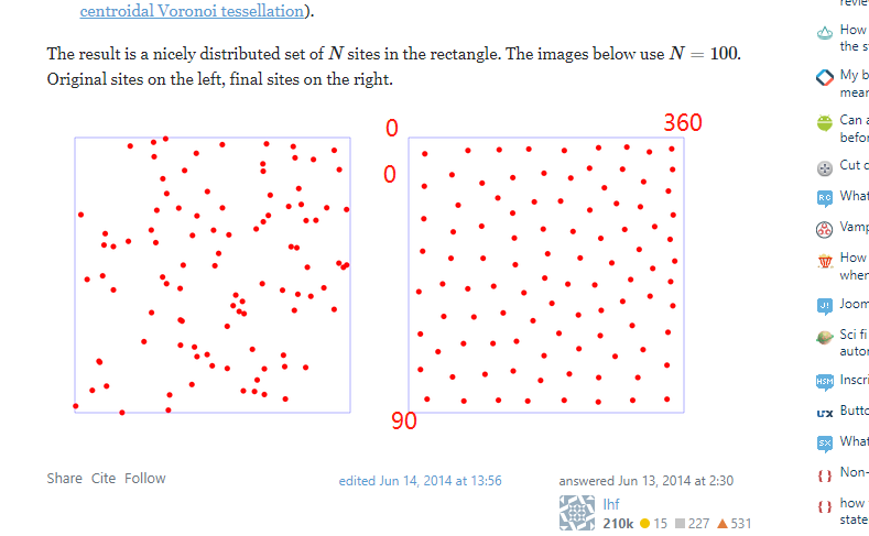
但并不适用于矩形上选择

突然发现一个很大的问题，我不能使用该方法来寻找星点，因为这种均匀分布是星点之间的角距的均匀分布，在观测时高度越高观测点越少，在高度低的地方观测点较多，其实并不适用于机架的校正。机架的校正应该按照经纬度网格来均匀选取。

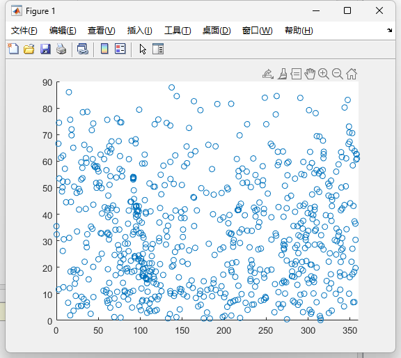
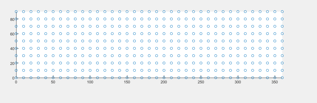
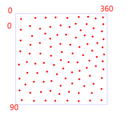
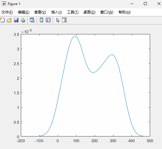
那么其实就可以将头顶的天区展开为一个矩形，方位和高度为边的矩形，研究在矩形上的二维均匀分布。

浅画一下二维的高度方位图（5等星

论文

Vedder, J.D.: ‘Star trackers, star catalog, and attitude determination: probabilistic aspects of system design’, J. Guid. Control Dyn., 1993, 16, (3), pp. 499–504

专利《用于星敏感器的筛选导航星的方法》

2004

在Stack Overflow中找到了我想问问题的答案

https://stackoverflow.com/questions/13005294/measure-the-uniformity-of-distribution-of-points-in-a-2d-square

通常在统计学中，我们需要了解给定的样本是否来自特定的分布，最常见的是正态分布(或高斯分布)。为此，我们有所谓的正态性检验，如夏皮罗-威尔克，安德森-达林或Kolmogorov-Smirnov检验。

它们都测量样本来自正态分布的可能性有多大，并有相关的p值来支持这种测量。

就是KS检验。Kolmogorov-Smirnov test是一个有用的非参数（nonparmetric）假设检验，主要是用来检验一组样本是否来自于某个概率分布（one-sample K-S test），或者比较两组样本的分布是否相同（two-sample K-S test）。

ks检验返回两个值，pvalue是越高越好，统计量D-statistic越低越好

值的解释

https://stats.stackexchange.com/questions/57885/how-to-interpret-p-value-of-kolmogorov-smirnov-test-python

https://en.m.wikipedia.org/wiki/Kolmogorov%E2%80%93Smirnov_test

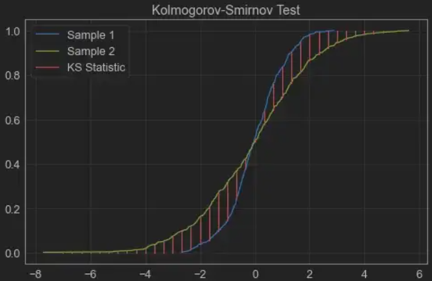
D 统计量是两个样本的 CDF 之间的绝对最大距离(最大值)。这个数字越接近于0，这两个样本就越有可能来自同一个分布。

K-s 检验返回的 p 值与其他 p 值具有相同的解释。如果 p 值小于你的显著性水平，那么你就拒绝了两个样本来自同一个分布的无效假设。如果您对该过程感兴趣，可以在线找到将 D 统计量转换为 p 值的表。

最终返回的结果，p-value=4.7405805465370525e-159，比指定的显著水平（假设为5%）小，则我们完全可以拒绝假设：beta和norm不服从同一分布。

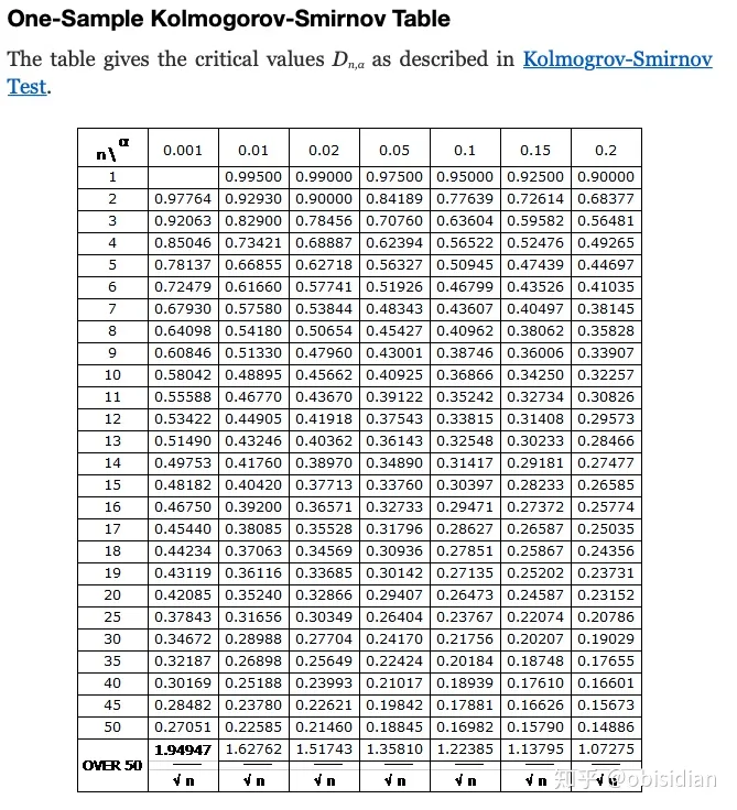
学习一下ks检验 柯尔莫哥洛夫-斯米尔诺夫检验（英语：Kolmogorov-Smirnov test，简称K-S test），是一种基于累计分布函数的非参数检验，用以检验两个经验分布是否不同或一个经验分布与另一个理想分布是否不同。

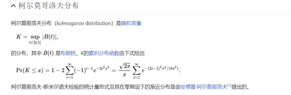
https://zhuanlan.zhihu.com/p/292678346

α是置信系数

https://zhuanlan.zhihu.com/p/26477641

from scipy.stats import ks_2samp
from scipy.stats import kstest
import numpy as np

norm1 = [105, 108, 111, 112, 113, 113, 117, 128, 130, 131]
print(norm1)
ks_value = kstest(norm1, 'norm', args=(120, 10))
print(ks_value)

KstestResult(statistic=0.35803634777692694, pvalue=0.11834016917515)

用一种简单的方式，我们可以将2样本检验的KS统计量D 定义为每个样本的cdf(累积分布函数)之间的最大距离，cdf 累计分布函数 https://towardsdatascience.com/comparing-sample-distributions-with-the-kolmogorov-smirnov-ks-test-a2292ad6fee5

from scipy.stats import kstest
import numpy as np
import matplotlib.pyplot as plt
norm1 = [0, 1, 2, 3, 4, 5, 6, 7, 8, 9, 10]
print(norm1)
ks_value = kstest(norm1, 'uniform', args=(0, 10), N=12)
[0, 1, 2, 3, 4, 5, 6, 7, 8, 9, 10]
KstestResult(statistic=0.09090909090909094, pvalue=0.9998600940511319)
print(ks_value)

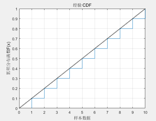
clc;clear;close all;
x = [1,2,3,4,5,6,7,8,9,10];
pd2 = makedist('Uniform','lower',0,'upper',10); % Uniform distribution with a = -2 and b = 2
t = 0:.01:10;
cdf2 = cdf(pd2, t);
h1 = cdfplot(x);
hold on
plot(t,cdf2,'k:','LineWidth',2);
xlabel('样本数据');
ylabel('累积分布函数F(x)');

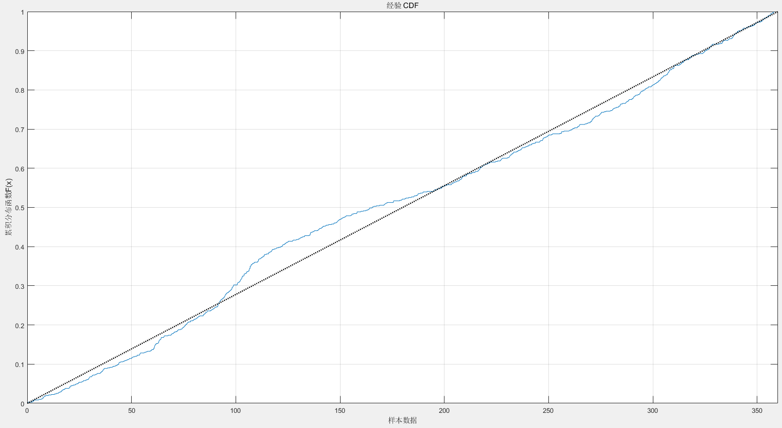
试试实时方位数据

from scipy.stats import kstest
import numpy as np
import matplotlib.pyplot as plt
import pandas as pd
user_cols = ['hip', 'az', 'alt', 'mag']
pd_reader = pd.read_csv("./J2000_5_hor.csv", header=None,
                        engine='python', index_col=0, usecols=list(range(4)), names=user_cols)
print(pd_reader.head())
norm1 = pd_reader['az']
print(norm1)
ks_value = kstest(norm1, 'uniform', args=(0, 360))
print(ks_value)

KstestResult(statistic=0.06621370056497172, pvalue=0.0038362399448040162)

实验感觉有问题 https://bbs.pinggu.org/thread-2983774-1-1.html

https://stats.stackexchange.com/questions/153249/non-uniform-distribution-of-p-values-when-simulating-binomial-tests-under-the-nu/

clc;clear;close all;
M = csvread('J2000_5_hor.csv');
x = M(:, 2);
pd2 = makedist('Uniform','lower',0,'upper',360); % Uniform distribution with a = -2 and b = 2
t = 0:.01:360;
cdf2 = cdf(pd2, t);
h1 = cdfplot(x);
hold on
plot(t,cdf2,'k:','LineWidth',2);
xlabel('样本数据');
ylabel('累积分布函数F(x)');
xlim([0 360])
ylim([0 1])

ks检验还是到此为止了，毕竟还只是个检验方法，不算指标

检验数据是否服从指定分布的方法有

https://blog.csdn.net/Datawhale/article/details/120558925

可知 KS检验的灵敏度没有相应的检验来的高

在该文中提到KL 散度是一种衡量两个概率分布的匹配程度的指标，两个分布差异越大，KL散度越大。KL越小越接近。

有人会把KL散度认为是一种距离指标，然而，KL散度不能用来衡量两个分布的距离。其原因在于KL散度不是对称的。举例来说，如果用观测分布来近似二项分布，其KL散度为

https://zhuanlan.zhihu.com/p/153492607

感觉不太合适，所以作罢

https://blog.csdn.net/qq_45654781/article/details/126862808

计算 Kozachenko-Leonenko的k最近邻估计熵

https://github.com/paulbrodersen/entropy_estimators

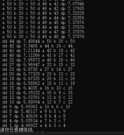
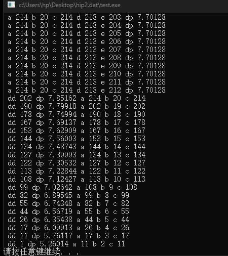
4等星 214个选20个

from scipy.special import gamma, digamma
import numpy as np
from entropy_estimators import continuous

# create some normal test data
# X = np.random.randn(20000, 1)

# X = np.arange(0, 0.09, 0.01)
# X = np.array([0, 1, 2, 3, 4, 5, 6, 7, 8, 9])
# X = np.array([189.83 195.095 195.192 196.886 198.814 203.376 204.429 218.318 227.266 261.36 301.009 308.907 345.333])
# dp 前a个点 选b个点 最后一次选的是c点 倒数第二次选的是d点
# dp[3][3][3][2] dp[4][4][4][3]
X = np.array([189.83, 261.36, 301.009, 345.333])
#            261-189  301-261 301-261  345-301

print(X.shape)
# compute the entropy from the determinant of the multivariate normal distribution:
analytic = continuous.get_h_mvn(X)

# compute the entropy using the k-nearest neighbour approach
# developed by Kozachenko and Leonenko (1,987):
kozachenko = continuous.get_h(X, k=1, norm='euclidean')

print(f"analytic result: {analytic:.5f}")
print(f"K-L estimator: {kozachenko:.5f}")
print(digamma(1))

运算时间很慢

用c++写dp（这个dp还没考虑球体的循环问题）

#include <bits/stdc++.h>
#include <boost/math/special_functions/digamma.hpp>
#pragma comment(linker, "/STACK:1073741824")
using namespace std;
// vector<double> points = {0.1, 1.2, 1.9, 2.3, 2.9, 3.9};
vector<double> points = {261.36, 345.333, 218.318, 196.886, 187.195, 187.387, 349.435, 262.478, 352.194, 186.59, 355.361, 358.033, 347.135, 179.794, 179.51, 178.597, 14.876, 172.61, 5.50809, 175.587, 158.055, 175.579, 18.0717, 18.0694, 167.389, 163.211, 98.636, 135.693, 10.1721, 131.4, 172.071, 152.177, 6.69029, 43.8872, 117.085, 72.1644, 168.928, 0.366764, 135.911, 94.3341, 29.6564, 158.157, 129.038, 35.8318, 65.4447, 60.8557, 52.6322, 150.143, 144.502, 44.7996, 117.286, 115.854, 133.016, 50.1732, 130.872, 78.2541, 92.0012, 59.5689, 91.4648, 91.6474, 91.4945, 78.2767, 64.2761, 130.576, 105.338, 112.139, 51.6668, 140.95, 98.267, 95.4699, 92.6435, 96.5942, 135.931, 94.7702, 114.749, 113.036, 102.779, 103.887, 106.395, 71.9267, 57.5453, 61.2187, 125.211, 60.8502, 110.887, 119.231, 112.454, 54.2793, 110.83, 105.955, 97.9926, 74.9688, 120.518, 102.988, 117.519, 93.22, 107.316, 103.157, 81.8369, 103.996, 103.994, 103.133, 119.554, 113.025, 108.66, 117.34, 92.8309, 111.149, 42.8763, 53.886, 62.5918, 76.2882, 75.3801, 100.752, 79.2899, 70.6052, 81.4649, 61.3945, 74.194, 69.2536, 63.5351, 58.963, 64.2205, 61.0484, 28.6315, 36.2729, 36.4375, 22.0025, 29.8624, 22.9935, 16.475, 13.928, 8.27138, 2.78788, 353.602, 352.709, 349.577, 342.741, 338.205, 337.806, 314.748, 325.078, 319.051, 327.003, 322.017, 303.285, 301.663, 340.939, 307.003, 300.783, 310.137, 299.254, 281.805, 334.071, 318.207, 269.96, 315.802, 291.564, 307.793, 273.792, 280.855, 336.666, 271.656, 268.879, 280.421, 260.389, 308.107, 249.547, 247.287, 300.084, 268.299, 270.919, 271.962, 305.234, 326.502, 291.083, 247.667, 299.381, 302.746, 284.357, 294.458, 328.324, 231.173, 338.978, 243.665, 233.148, 324.253, 256.191, 232.279, 216.426, 241.766, 272.257, 208.418, 247.348, 325.249, 237.343, 236.978, 314.613, 245.759, 203.524, 276.607, 200.523, 339.604, 265.049, 224.551, 218.172, 209.523, 302.305, 269.956, 245.845, 211.412, 227.112, 317.642, 353.915};
// vector<double> points(point.begin(), point.begin() + 50);
double log_c_d = (1 / 2.) * log(M_PI) - log(tgamma(1 / 2. + 1));
double func(int j, int k)
{
    double distances = points[j - 1] - points[k - 1];
    double sum_log_dist = 2 * log(2 * distances);
    double h = -boost::math::digamma(1) + boost::math::digamma(2) + log_c_d + (1 / 2.0) * sum_log_dist;
    return h;
}
int main()
{
    int n = points.size();
    int m = 20;
    cout << " n " << n << endl;
    sort(points.begin(), points.end());
    for (double num : points)
        cout << num << " ";
    cout << endl;

    // double dp[51][21][51][51];
    // memset(dp, 0, sizeof(dp));
    vector<vector<vector<vector<double>>>> dp(n + 1, vector<vector<vector<double>>>(m + 1, vector<vector<double>>(n + 1, vector<double>(n + 1))));

    cout << " 1";
    for (int i = 2; i <= n; i++)
        for (int k = i - 1; k >= 1; k--)
            dp[i][2][i][k] = func(i, k);

    for (int a = 3; a <= n; a++)
        for (int b = 2; b <= m; b++)
            for (int c = b; c <= a; c++)
                for (int d = b - 1; d <= a - 1 && d <= c - 1; d++)
                {
                    if (c == a && b == 2)
                        continue;
                    if (c != a)
                    { // 没选a
                        dp[a][b][c][d] = dp[a - 1][b][c][d];//120^4 * 20 dp 前a个点 选b个点 最后一次选的是c点 倒数第二次选的是d点  筛选问题 700 选 50 
                    }
                    else
                    {
                        for (int e = b - 2; e <= d - 1; e++)
                        {
                            double last = dp[a - 1][b - 1][d][e];
                            double newv = ((last + boost::math::digamma(1) - boost::math::digamma(b - 1) - log_c_d) * (b - 1) - log(2 * (points[d - 1] - points[e - 1])) + log(2 * (points[c - 1] - points[d - 1])) + log(2 * min(points[c - 1] - points[d - 1], points[d - 1] - points[e - 1]))) / double(b) - boost::math::digamma(1) + boost::math::digamma(b) + log_c_d;
                            // if ( a == 4 && b == 3 && c)
                            dp[a][b][c][d] = max(dp[a][b][c][d], newv);
                            cout << " a " << a << " b " << b << " c " << c << " d " << d << " e " << e << " dp " << dp[a][b][c][d] << endl;
                        }
                    }
                }

    // double maxv = 0.0;
    // int a = 13, b = 4;
    // int cc, dd;
    // // while (d > 1)
    // {
    //     for (int c = b; c <= a; c++)
    //         for (int d = b - 1; d <= a - 1 && d <= c - 1; d++)
    //             if (dp[a][b][c][d] > maxv)
    //             {
    //                 maxv = dp[a][b][c][d];
    //                 cc = c;
    //                 dd = d;
    //             }
    //     cout << " cc " << cc << " dd " << dd << " dp " << maxv << endl;
    // }

    double maxv = 0.0;

    int a = n, b = m, c = a;
    int dd = 2;
    while (dd > 1)
    {
        for (int d = c - 1; d >= b - 1; d--)
        {
            if (dp[a][b][c][d] > maxv)
            {
                maxv = dp[a][b][c][d];
                dd = d;
            }
        }
        cout << " dd " << dd << " dp " << maxv << " a " << a << " b " << b << " c " << c << endl;
        a = dd;
        c = a;
        maxv = 0.0;
        b--;
    }

    system("pause");
    return 0;
}

采用模拟退火进行加速运算

https://www.bilibili.com/video/BV1hK41157JL/?spm_id_from=333.337.search-card.all.click&vd_source=6c92aa3e5d0f2e0347ec135013a906d8

b站教程不错

选用第三个例题《书店买书》的案例

https://mp.weixin.qq.com/s/001Klrt7jjf8s5rI3py7Yg

clear all;close all; clc;
points = [261.36,345.333,218.318,196.886,187.195,187.387,349.435,262.478,352.194,186.59,355.361,358.033,347.135,179.794,179.51,178.597,14.876,172.61,5.50809,175.587,158.055,175.579,18.0717,18.0694,167.389,163.211,98.636,135.693,10.1721,131.4,172.071,152.177,6.69029,43.8872,117.085,72.1644,168.928,0.366764,135.911,94.3341,29.6564,158.157,129.038,35.8318,65.4447,60.8557,52.6322,150.143,144.502,44.7996,117.286,115.854,133.016,50.1732,130.872,78.2541,92.0012,59.5689,91.4648,91.6474,91.4945,78.2767,64.2761,130.576,105.338,112.139,51.6668,140.95,98.267,95.4699,92.6435,96.5942,135.931,94.7702,114.749,113.036,102.779,103.887,106.395,71.9267,57.5453,61.2187,125.211,60.8502,110.887,119.231,112.454,54.2793,110.83,105.955,97.9926,74.9688,120.518,102.988,117.519,93.22,107.316,103.157,81.8369,103.996,103.994,103.133,119.554,113.025,108.66,117.34,92.8309,111.149,42.8763,53.886,62.5918,76.2882,75.3801,100.752,79.2899,70.6052,81.4649,61.3945,74.194,69.2536,63.5351,58.963,64.2205,61.0484,28.6315,36.2729,36.4375,22.0025,29.8624,22.9935,16.475,13.928,8.27138,2.78788,353.602,352.709,349.577,342.741,338.205,337.806,314.748,325.078,319.051,327.003,322.017,303.285,301.663,340.939,307.003,300.783,310.137,299.254,281.805,334.071,318.207,269.96,315.802,291.564,307.793,273.792,280.855,336.666,271.656,268.879,280.421,260.389,308.107,249.547,247.287,300.084,268.299,270.919,271.962,305.234,326.502,291.083,247.667,299.381,302.746,284.357,294.458,328.324,231.173,338.978,243.665,233.148,324.253,256.191,232.279,216.426,241.766,272.257,208.418,247.348,325.249,237.343,236.978,314.613,245.759,203.524,276.607,200.523,339.604,265.049,224.551,218.172,209.523,302.305,269.956,245.845,211.412,227.112,317.642,353.915];

points = sort(points);

chose = int16([1 12 15 50 60 89 98 99 106 124 126 131 133 134 150 151 165 202 206 207]);
chose = sort(chose);

scatter(points,0,'k.');
hold on;
for s = chose
    disp(s);
    scatter(points(s), 0,'red','filled');
    hold on;
end

初始方案是：
[1 12 15 50 60 89 98 99 106 124 126 131 133 134 150 151 165 202 206 207]
此时最优值是：
46.3648

最佳的方案是：
[7 15 21 28 42 53 60 78 96 105 109 118 127 137 150 166 176 190 203 214]
此时最优值是：
93.4483

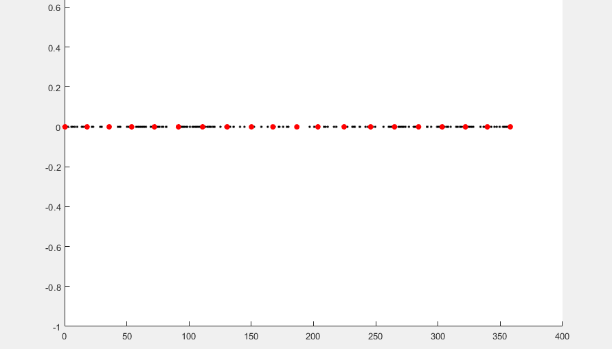
初始点：

优化方案：

%% 模拟退火解决书店买书问题  % 466
clear all; clc; close all;
% tic
load points;
points = sort(points);
rng('shuffle')  % 控制随机数的生成，否则每次打开matlab得到的结果都一样
len = 20;
map = [1:len,1:len];
% 这个数据文件里面保存了两个矩阵：M是每本书在每家店的价格; freight表示每家店的运费
% [s, b] = size(M);  % s是书店的数量，b是要购买的书的数量

%% 参数初始化
T0 = 1000;   % 初始温度
T = T0; % 迭代中温度会发生改变，第一次迭代时温度就是T0
maxgen = 500;  % 最大迭代次数
Lk = 200;  % 每个温度下的迭代次数
alfa = 0.95;  % 温度衰减系数

%%  随机生成一个初始解
A = int32(1:length(points));
random_num = A(randperm(numel(A),len));
index0 = sort(random_num);
h0 = Copy_of_totalH(points, index0, len);

% way0 = randi([1, s],1,b); % 在1-s这些整数中随机抽取一个1*b的向量，表示这b本书分别在哪家书店购买
% money0 = calculate_money(way0,freight,M,b); % 调用我们自己写的calculate_money函数计算这个方案的花费
disp('初始方案是：'); disp(mat2str(index0))
disp('此时最优值是：'); disp(h0)
%% 定义一些保存中间过程的量，方便输出结果和画图
min_money = h0;     % 初始化找到的最佳的解对应的花费为money0
MONEY = zeros(maxgen,1); % 记录每一次外层循环结束后找到的min_money (方便画图）

%% 模拟退火过程
for iter = 1 : maxgen  % 外循环, 我这里采用的是指定最大迭代次数
    for i = 1 : Lk  %  内循环，在每个温度下开始迭代
        index = index0;
        x_num = index(randperm(numel(index),1));
        x = find(index == x_num);
   
        delta = 0;
        delta = delta ...
            - log(2* min( mod(points(index(map(x-1+len)))-points(index(map(x-2+len))) + 360, 360), mod( points( index(x)) - points(index(map(x-1+len))) + 360, 360) )) ...
            - log(2* min( mod(points(index(x)) - points(index(map(x-1+len))) + 360 , 360) , mod( points(index(map(x+1))) - points(index(x)) + 360 , 360 ) )) ...
            - log(2* min( mod(points(index(map(x+1))) - points(index(x)) + 360 , 360), mod(points(index(map(x+2))) - points(index(map(x+1))) + 360, 360 ) )) ...
            + log(2* min( mod(points(index(map(x-1+len))) - points(index(map(x-2+len))) + 360, 360), mod(points(index(map(x+1))) - points(index(map(x-1+len))) + 360, 360) )) ...
            + log(2* min( mod(points(index(map(x+2))) - points(index(map(x+1))) + 360, 360), mod(points(index(map(x+1))) - points(index(map(x-1+len))) + 360, 360) ));
        
        
        shengxia = setxor(A, index);
        y_num = shengxia(randperm(numel(shengxia),1));
        index(x) = y_num;
        index = sort(index);
        y = find(index == y_num);
        delta = delta ...
            - log(2* min( mod(points(index(map(y-1+len)))-points(index(map(y-2+len))) + 360, 360), mod( points( index(map(y+1))) - points(index(map(y-1+len))) + 360, 360) )) ...
            - log(2* min( mod(points(index(map(y+1))) - points(index(map(y-1+len))) + 360 , 360) , mod( points(index(map(y+2))) - points(index(map(y+1))) + 360 , 360 ) )) ...
            + log(2* min( mod(points(index(map(y-1 + len))) - points(index(map(y-2+len))) + 360 , 360), mod(points(index(y)) - points(index(map(y-1 + len))) + 360, 360 ) )) ...
            + log(2* min( mod(points(index(y)) - points(index(map(y-1+len))) + 360, 360), mod(points(index(map(y+1))) - points(index(y)) + 360, 360) )) ...
            + log(2* min( mod(points(index(map(y+1))) - points(index(y)) + 360, 360), mod(points(index(map(y+2))) - points(index(map(y+1))) + 360, 360) ));
        
        index1 = index;  % 调用我们自己写的gen_new_way函数生成新的方案
        
        if delta > 0    % 如果新方案的花费小于当前方案的花费
            index0 = index1; % 更新当前方案为新方案
            h0 = h0 + delta;
        else
%             p = exp(-(money1 - money0)/T); % 根据Metropolis准则计算一个概率
            p = exp(delta/T); % 根据Metropolis准则计算一个概率
            if rand(1) < p   % 生成一个随机数和这个概率比较，如果该随机数小于这个概率
                index0 = index1; % 更新当前方案为新方案
                h0 = h0 + delta;
            end
        end
        % 判断是否要更新找到的最佳的解
        if h0 > min_money  % 如果当前解更好，则对其进行更新
            min_money = h0;  % 更新最大的花费
            best_way = index1;  % 更新找到的最佳方案
        end
    end
    MONEY(iter) = min_money; % 保存本轮外循环结束后找到的最小花费
    T = alfa*T;   % 温度下降
end

disp('最佳的方案是：'); disp(mat2str(best_way))
disp('此时最优值是：'); disp(min_money)

%% 画出每次迭代后找到的最佳方案的图形
figure
plot(1:maxgen,MONEY,'b-');
xlabel('迭代次数');
ylabel('最小花费');
% toc

用py验证一下

改变一下distance的定义，由于要循环

def get_h(x, k=1, norm='max', min_dist=0.):
    n, d = x.shape

    p = 2
    log_c_d = (d/2.) * log(np.pi) - log(gamma(d/2. + 1))
    print(log_c_d)

    kdtree = cKDTree(x)

    distances, _ = kdtree.query(x, k + 1, eps=0, p=p)
    distances = distances[:, -1]
    distances[0] = min(x[1] - x[0], x[0] + 360 - x[-1])
    distances[-1] = min(x[-1] - x[-2], x[0] + 360 - x[-1])
    print("distance", distances)
    # enforce non-zero distances
    distances[distances < min_dist] = min_dist
    # where did the 2 come from? radius -> diameter
    sum_log_dist = np.sum(log(2*distances))
    h = sum_log_dist

    return h

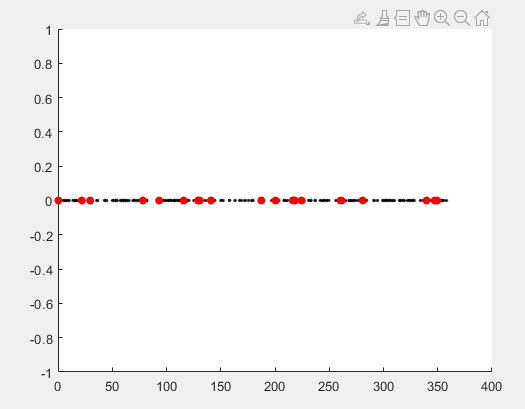
初始方案是：
[26 27 36 38 52 64 69 77 86 102 132 149 150 154 156 157 173 187 199 201]
此时最优值是：
26.7911

最佳的方案是：
[5 12 19 27 44 57 87 103 110 120 126 132 138 147 152 165 172 188 198 210]
此时最优值是：
70.6790

历时 3.124118 秒。

迭代计算只需要计算那改变的6个点，试试直接计算h0 看时间会多慢

%% 模拟退火解决书店买书问题  % 466
clear all; clc; close all;
tic
load points;
points = sort(points);
rng('shuffle')  % 控制随机数的生成，否则每次打开matlab得到的结果都一样
len = 20;
map = [1:len,1:len];
% 这个数据文件里面保存了两个矩阵：M是每本书在每家店的价格; freight表示每家店的运费
% [s, b] = size(M);  % s是书店的数量，b是要购买的书的数量

%% 参数初始化
T0 = 1000;   % 初始温度
T = T0; % 迭代中温度会发生改变，第一次迭代时温度就是T0
maxgen = 500;  % 最大迭代次数
Lk = 200;  % 每个温度下的迭代次数
alfa = 0.95;  % 温度衰减系数

%%  随机生成一个初始解
A = int32(1:length(points));
random_num = A(randperm(numel(A),len));
index0 = sort(random_num);
h0 = Copy_of_totalH(points, index0, len);

% way0 = randi([1, s],1,b); % 在1-s这些整数中随机抽取一个1*b的向量，表示这b本书分别在哪家书店购买
% money0 = calculate_money(way0,freight,M,b); % 调用我们自己写的calculate_money函数计算这个方案的花费
disp('初始方案是：'); disp(mat2str(index0))
disp('此时最优值是：'); disp(h0)
%% 定义一些保存中间过程的量，方便输出结果和画图
min_money = h0;     % 初始化找到的最佳的解对应的花费为money0
MONEY = zeros(maxgen,1); % 记录每一次外层循环结束后找到的min_money (方便画图）

%% 模拟退火过程
for iter = 1 : maxgen  % 外循环, 我这里采用的是指定最大迭代次数
    for i = 1 : Lk  %  内循环，在每个温度下开始迭代
        index = index0;
        x_num = index(randperm(numel(index),1));
        x = find(index == x_num);
        shengxia = setxor(A, index);
        y_num = shengxia(randperm(numel(shengxia),1));
        index(x) = y_num;
        index = sort(index);      
        index1 = index;  % 调用我们自己写的gen_new_way函数生成新的方案

        h1 = Copy_of_totalH(points, index1, len);

        if h1 > h0    % 如果新方案的花费小于当前方案的花费
            index0 = index1; % 更新当前方案为新方案
            h0 = h1;
        else
%             p = exp(-(money1 - money0)/T); % 根据Metropolis准则计算一个概率
            p = exp((h1 - h0)/T); % 根据Metropolis准则计算一个概率
            if rand(1) < p   % 生成一个随机数和这个概率比较，如果该随机数小于这个概率
                index0 = index1; % 更新当前方案为新方案
                h0 = h1;
            end
        end
        % 判断是否要更新找到的最佳的解
        if h0 > min_money  % 如果当前解更好，则对其进行更新
            min_money = h0;  % 更新最大的花费
            best_way = index1;  % 更新找到的最佳方案
        end
    end
    MONEY(iter) = min_money; % 保存本轮外循环结束后找到的最小花费
    T = alfa*T;   % 温度下降
end

disp('最佳的方案是：'); disp(mat2str(best_way))
disp('此时最优值是：'); disp(min_money)

%% 画出每次迭代后找到的最佳方案的图形
figure
plot(1:maxgen,MONEY,'b-');
xlabel('迭代次数');
ylabel('最小花费');
toc

历时 3.305654 秒。

但耗时也不多

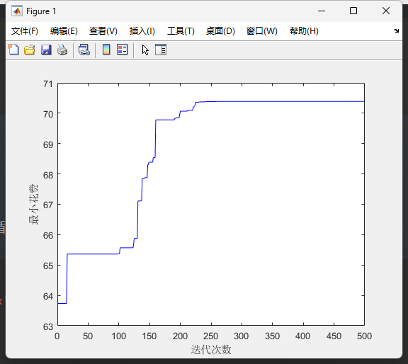
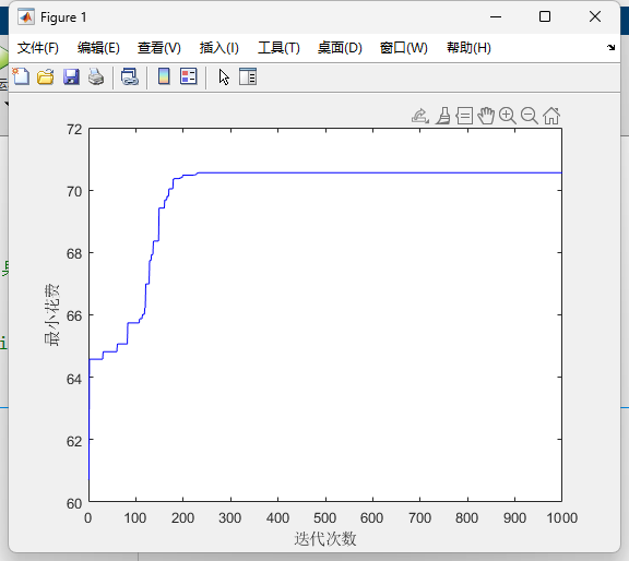
但增加迭代次数

maxgen = 1000; % 最大迭代次数
Lk = 1000; % 每个温度下的迭代次数

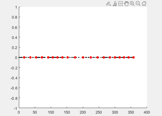
初始方案是：
[10 26 35 62 76 77 91 120 129 130 141 151 163 166 176 180 182 208 209 214]
此时最优值是：
43.8157

最佳的方案是：
[10 17 23 40 53 67 90 105 110 120 126 131 138 148 153 166 172 188 200 214]
此时最优值是：
70.7798

历时 31.648947 秒。

而只用6个点的数据

历时 29.961089 秒。

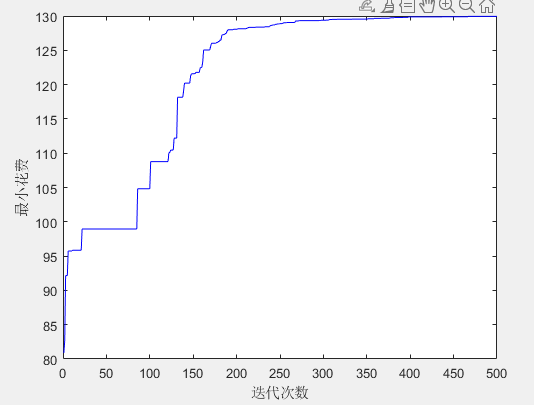
708个点选50个点也只需要4s

初始方案是：
[7 32 33 83 98 103 106 113 139 152 161 164 171 201 220 229 235 257 280 298 299 319 332 349 352 355 360 365 373 393 401 407 434 450 455 470 479 506 508 531 540 548 565 566 589 603 640 679 689 707]
此时最优值是：
73.5312

最佳的方案是：
[12 26 39 52 64 74 82 93 119 132 151 166 184 208 230 255 271 285 296 305 320 329 342 350 359 367 379 389 406 427 439 455 466 474 486 492 503 519 530 544 561 577 598 615 630 639 651 672 686 708]
此时最优值是：
130.3724

历时 4.013932 秒。