均匀性-玻尔兹曼熵
在多篇文章中提到玻尔兹曼熵来表征评价均匀性(还有各分区内的星数标准差)。


多尺度像面分割《CN201510107562.0-用于星敏感器的筛选导航星的方法》
玻尔兹曼熵《Boltzmann entropy-based guide star selection algorithm for star tracker》2005
正交网格法《A general method of the automatical selection of guide star》
用到uniformity的计算
均匀性计算《Star trackers, star catalogs, and attitude determination-Probabilistic aspects of system design》1993
《基于螺旋基准点的导航星选取方法》
均匀性很好


clear all ;close all; |

后来我又看到 https://zhuanlan.zhihu.com/p/25988652?group_id=828963677192491008 菲波那契网格
clear all ;close all; |

效果并不好

阿基米德螺旋线

clear all; close all; |

弧长公式 https://www.zhihu.com/question/27384632
《均匀快速的导航星选取方法》
在赤纬带平分点,矩形范围的代码见下。(两角和余弦公式)


《16mv精细导星星库构建与评价》
分区后取最亮几个。
国内研究构建星库的方法主要分为两类:第一类从星表划分角度出发,通过不同的划分方式进行导星筛选,现有的星表划分方法主要有赤纬带法、圆锥法、球矩形法、内接正方体法等;第二类从局部天区出发,主要包括回归筛星法、星等加权算法等。
评价标准:完备性 、均匀性和冗余性。(均匀性、速度、多于3个星的分区数概率)


《适用于小视场星敏感器的导航星表构建方法》

在1993年的均匀性计算文章中提到这一计算方法
总体均匀性计算方法:


局部均匀性计算方法:

以上一篇《基于星座聚类的星敏感器导航星优选算法研究》为例,
所有4908个点的全局均匀性为
% boltzmannEntropy.m |
newmatrix =
0.2799 -0.0070 0.0483
-0.0070 0.3631 0.0007
0.0483 0.0007 0.3570
eigen =
0.2562
0.3632
0.3805
ans =
0.0142
均匀化后 得到39个点 data=
clear |
0.721096202739022 0.143274305623194 -0.677858937938827
0.968970810392417 0.208978537391637 0.131998255735122
0.569826352357379 0.276879108656515 0.773715637265177
0.228610689351435 0.164381998103028 -0.959539322494872
0.680467391588214 0.574452415904999 0.454937963733565
0.755501580234282 0.652710692710075 0.0564456719814448
0.504277122250002 0.768039960865827 -0.394739410863010
0.154912237007631 0.405692531666614 0.900786194707282
0.210384928706513 0.600544339596624 -0.771417317637872
0.143977198200687 0.816855223274374 0.558585813109905
-0.229099414143074 0.950795223816936 -0.208571092930452
-0.282616508078908 0.919125613504918 0.274474071563222
-0.273028245935124 0.599816587126275 0.752114112837791
-0.384654835774312 0.742153343311259 -0.548861614915233
-0.256254169146301 0.406094432070341 -0.877166525259945
-0.739931959521445 0.571829210408285 -0.354276797719793
-0.806338802865188 0.579353885367924 0.119024411374415
-0.760075452992603 0.337837739926240 0.555113472399671
-0.487550601625308 0.150466743789691 0.860031493532724
-0.987416677336434 0.156220148544471 0.0245676719820876
-0.898581139351745 -0.0465144783456416 0.436335122704501
-0.374139568095630 -0.0287413085026819 -0.926926923101692
-0.963578273457490 -0.260891712855464 -0.0587573406820316
-0.799916216534544 -0.556325600463240 0.225024160467884
-0.732478694296601 -0.536144597346316 -0.419552062487963
-0.478334336301847 -0.740621679799566 0.471885356973005
-0.194005559456996 -0.435699798511738 0.878935451826020
-0.314232785230549 -0.886073947077770 -0.340779572445699
-0.00720050076528926 -0.0591052787344646 0.998225785488659
-0.0490019433066575 -0.732931424546231 -0.678535434936750
0.0801942976395903 -0.872038194549829 0.482823220104800
0.368597406332163 -0.929570349282381 0.00590912685900466
0.323982389195822 -0.553545295684837 0.767217711680429
0.514345456211916 -0.579655346834382 -0.632019327679517
0.827337679920563 -0.510494571429276 -0.234323827053289
0.448212896485379 -0.212583754752496 -0.868281835949317
0.964675223452813 -0.215965114222275 0.150866771342216
0.724877321462857 -0.104703930494290 0.680874405281827
0.927771336185871 -0.108671846203537 -0.356974477511487

newmatrix =
0.3527 -0.0057 -0.0221
-0.0057 0.3007 0.0039
-0.0221 0.0039 0.3466
eigen =
0.3001
0.3273
0.3726
ans =
0.0040
均匀性不错。
又做一次实验
newmatrix =
0.3364 -0.0062 -0.0127
-0.0062 0.3195 0.0007
-0.0127 0.0007 0.3441
eigen =
0.3169
0.3290
0.3541
ans =
0.0011

随机选取39个点
clc;clear;close all; |
newmatrix =
0.3068 -0.0422 0.0801
-0.0422 0.3637 -0.0381
0.0801 -0.0381 0.3295
eigen =
0.2368
0.3226
0.4406
ans =
0.0314

% 矩形范围 |